Lately I'm playing around with Recursive Bayesian estimators (http://en.wikipedia.org/wiki/Recursi...ian_estimation) for which the Kalman filter is a special case. I won't enter in the gory details; see Bayesian Forecasting and Dynamic Models by West and Harrison.
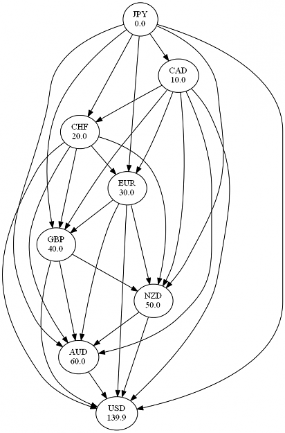
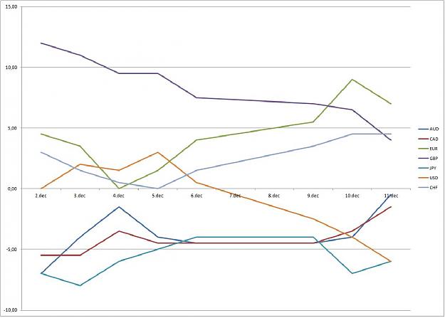
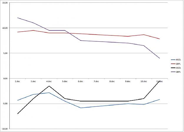
At first I was trying to estimate the trend and the volatility of the market... But that's not what this post is about. It is about why you'd better off be long on the Dragon today.
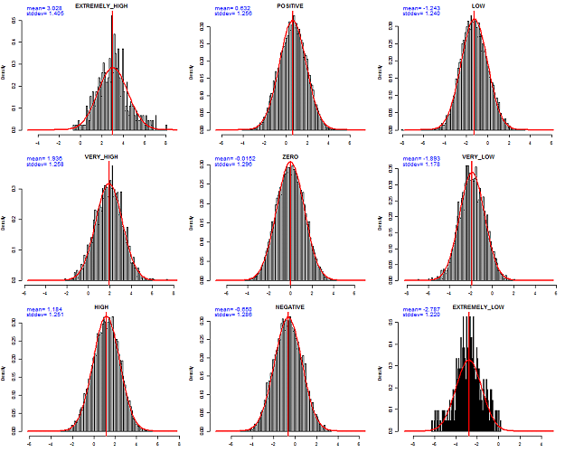
The market return is not Normally distributed but somewhere between Cauchy and Student distributed. Kalman filter performances degrade quickly for non-Normal innovations. That's why I use another Kalman filter which estimates the error of the first one and I feedback this information into the first model as a modulation of the allowed variance of the state. A kind of dynamic cursor "lag <-> smoothness".
This first model is a second order polynomial local estimation. I chose a 2nd order polynomial because it can approximate (Taylor) any smooth function like a sine wave for a market with a cyclic component (range or valatile trend) or an exponential trend (for index and stocks). Also the accelaration factor helps catching up with the price in case of a sudden move. The second filter just uses a constant model. I use H4 to gauge the daily trend.
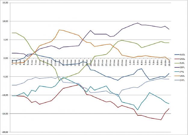
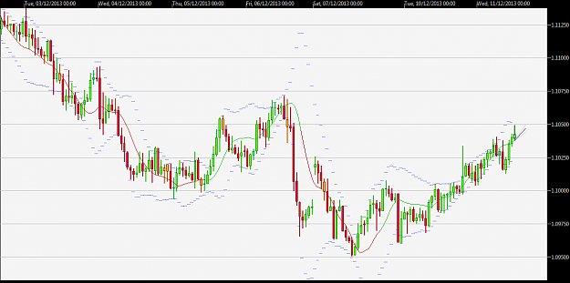
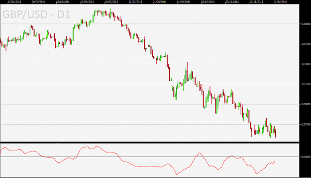
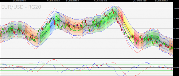
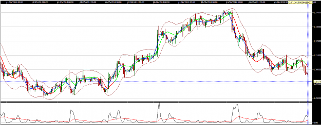
Here is a screenshot of EUR/USD H4. The blue line is the ideal, but non-causal, low pass filter sinc (http://en.wikipedia.org/wiki/Sinc_filter) used with 41 samples. It gives you an idea of the lag. The filter is green when the trend is most likely up and red otherwise. The dash envelope is the 95% confidence interval of the mean price estimate. Below are the error between the price and the estimate (black) and this value filtered with the 2nd filter (red). It doesn't follow the error too much to not make the main filter over-react.
At first I was trying to estimate the trend and the volatility of the market... But that's not what this post is about. It is about why you'd better off be long on the Dragon today.
The market return is not Normally distributed but somewhere between Cauchy and Student distributed. Kalman filter performances degrade quickly for non-Normal innovations. That's why I use another Kalman filter which estimates the error of the first one and I feedback this information into the first model as a modulation of the allowed variance of the state. A kind of dynamic cursor "lag <-> smoothness".
This first model is a second order polynomial local estimation. I chose a 2nd order polynomial because it can approximate (Taylor) any smooth function like a sine wave for a market with a cyclic component (range or valatile trend) or an exponential trend (for index and stocks). Also the accelaration factor helps catching up with the price in case of a sudden move. The second filter just uses a constant model. I use H4 to gauge the daily trend.
Here is a screenshot of EUR/USD H4. The blue line is the ideal, but non-causal, low pass filter sinc (http://en.wikipedia.org/wiki/Sinc_filter) used with 41 samples. It gives you an idea of the lag. The filter is green when the trend is most likely up and red otherwise. The dash envelope is the 95% confidence interval of the mean price estimate. Below are the error between the price and the estimate (black) and this value filtered with the 2nd filter (red). It doesn't follow the error too much to not make the main filter over-react.
Attached Image (click to enlarge)
No greed. No fear. Just maths.